How to Design and Build a Gas Dynamic Laser

Introduction

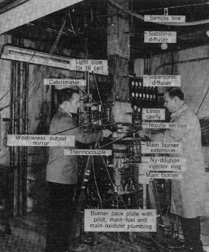
In the 1970s, gripped in the heart of the Cold War, American and Soviet scientists pushed the boundaries of the laws of physics to design advanced weapons and countermeasures to try and gain the upper hand. From even the first days after the invention of the first laser both sides raced to build more and more powerful lasers to fuel powerful directed energy weapons to gain an upper hand in a theoretical nuclear exchange that thankfully never came to pass. Among this early mania to design the most powerful lasers ever made the Gas Dynamic Laser was invented, a unique and bizarre form of laser that resembles a rocket engine more than a traditional laser. Born out of the same physics and laboratory used to develop the heat shields used in the Apollo program the GDL appears to break all the rules of lasers; achieving a population inversion through pure thermodynamics, powered purely by combustion, and able to achieve power densities beyond anything else.

While today it has been superseded by simpler fiber lasers and more powerful chemical lasers, I have been fascinated by this bizarre laser architecture for years. Given modern advances in manufacturing processes and computing, as well as a burgeoning liquid rocketry community, I believe that today it is perfectly achievable for a hobbyist to build one of these on their own. What follows is a short overview of my research as well as some advice and guidelines for constructing your own GDL.

Physics

The physics behind gas dynamic lasers are simultaneously what makes them interesting to me as well as what has made them historically so hard to design. A gas dynamic laser combines multiple disparate fields of physics which rarely interact including aerodynamics, thermodynamics, electromagnetism and optics, as well as a healthy dose of mechanical engineering to build one.

I will try to make my brief explanation as approachable as possible to anyone, however it is recommended that one have at least a background in physics if you really want to understand the underlying physical processes. My explanation will be by no means exhaustive and if you want a more definitive in-depth source I would heavily recommend Anderson's excellent 1976 text^[1].

Basics of Gas Lasers

To understand a gas dynamic laser one must first understand the simpler model of a gas laser. Luckily the most common form of gas dynamic laser is a CO₂–N₂ based laser, which shares many of the same physical properties as the common CO₂ laser used often for hobby and professional laser cutters.

Population Inversion

Every laser, no matter how exotic, relies on the same principle: Given a collection of atoms or molecules with quantized energy levels (either the energy levels of electrons in an atom's orbit, or the vibrational modes of a molecule), if one can push more of the said states into a higher level than a lower level they will amplify and intensify light energy as it passes through the medium.

This amplification effect is known as stimulated emission, an effect Einstein predicted in 1917 and the one that gives the laser its acronym (Light Amplification by Stimulated Emission of Radiation). When a molecule sits in an excited state and a photon of the right wavelength which exactly matches the energy of that state passes by, the photon can stimulate the molecule to drop down to a lower state and emit a second photon, identical in frequency, phase, and direction to the first. If one were to create a bulk material of molecules in this state you would have a system which would exponentially amplify any light which passed through it.

The catch is that the reverse process, absorption can also happen: a passing photon can just as easily be swallowed by a molecule sitting in the lower state, kicking it up to the excited one and converting that photon into potential energy stored in the molecule. In a normal gas at thermal equilibrium there are always more molecules in the lower state than the upper one, so absorption wins and a beam of light is attenuated rather than amplified. The relative populations of two states separated by an energy gap $\Delta E$ at a temperature $T$ follow the Boltzmann distribution:

$\frac{N_{upper}}{N_{lower}} = \exp\left(-\frac{\Delta E}{k_B T}\right)$

Since the exponent is always negative for a gas in equilibrium, the upper state is always less populated than the lower one. To get net amplification you need to flip this around so that the upper state is more populated than the lower state, a condition called a population inversion. Notice that no positive, finite temperature can ever satisfy this in equilibrium; a population inversion is fundamentally a non-equilibrium state, and achieving and maintaining one is the central problem of every laser. In fact in early laser literature this state is known as negative temperature (a more evocative, if less self explanatory name for the state).

CO₂ Lasers

When most people picture a laser they imagine electrons jumping between energy levels in an atom, as in a helium-neon or ruby laser. Afterall that is the traditional first explanation any undergrad would encounter. But molecules can store energy in other ways too. A molecule made of two or more atoms can rotate, and crucially it can vibrate, with its atoms oscillating back and forth as if connected by tiny springs. These vibrations are also quantized, meaning the molecule can only vibrate with certain discrete amounts of energy, and the gaps between these vibrational energy levels happen to correspond to photons in the infrared part of the spectrum.

A vibrational laser is simply a laser whose population inversion lives between two of these molecular vibrational states rather than between electronic states. Instead of emitting photons through the energy released by an electron moving from a higher orbital to a lower orbital, instead all the energy is released through vibrational transitions, molecules moving from a higher to lower vibrational mode and emitting a photon in the process. This does not occur in all molecules; intuitively an inert diatomic molecule such as N₂ would not be able to emit a photon as the individual atoms in the molecule have the exact same charge, thus there is no moving potential to create an EM field. Instead you need particular molecular transitions which are able to emit a photon, and these can be found in molecules such as carbon dioxide.

The carbon dioxide laser is the most important vibrational laser ever built, and it is the molecule at the heart of nearly every gas dynamic laser. A CO₂ molecule is linear, a carbon atom flanked by two oxygens, and it has three distinct ways to vibrate, called its normal modes:

• The symmetric stretch, where both oxygen atoms move outward and inward together.
• The bending mode, where the molecule flexes away from a straight line.
• The asymmetric stretch, where one oxygen moves in while the other moves out.

The asymmetric stretch mode is the special one. A molecule excited into this mode sits at a relatively high vibrational energy, and it can drop down into the symmetric stretch (or the bending mode) while emitting a photon. The transition from the asymmetric stretch down to the symmetric stretch produces the famous 10.6 μm infrared line that CO₂ lasers are known for. So if we can arrange for more CO₂ molecules to be sitting in the asymmetric stretch state than in the symmetric stretch state, we have our population inversion and we have a laser.

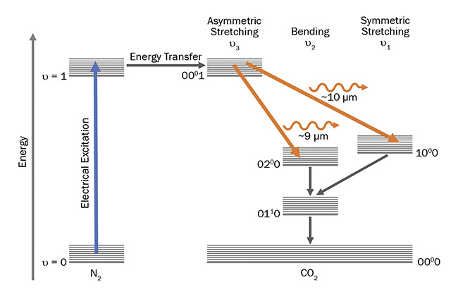
There are two features of CO₂ that make this practical. First, the upper laser level (the asymmetric stretch) is long lived, meaning a molecule will happily sit there for a relatively long time before spontaneously decaying, giving us time to build up a large population. Second, the lower laser level empties quickly, draining away through collisions so it does not clog up and destroy the inversion. A long lived upper level and a fast draining lower level are the ideal recipe for a population inversion.

In practice CO₂ lasers almost never use pure carbon dioxide. They use a mixture, and the most important additive is nitrogen (N₂). Nitrogen is a simple diatomic molecule with a single vibrational mode, and by a fortunate coincidence of nature the energy of its first vibrational level is almost exactly equal to the energy of the CO₂ asymmetric stretch. This near perfect match means that an excited nitrogen molecule colliding with a ground state CO₂ molecule can hand over its vibrational energy almost losslessly, kicking the CO₂ straight into its upper laser level. Nitrogen therefore acts as an energy reservoir and a pump: it is easy to excite in bulk, it holds that energy for a long time because a lone N₂ molecule has no easy way to radiate it away, and it feeds it efficiently into the CO₂. Additionally, most CO₂ lasers also contain small amounts of diluents, either H₂O or helium, whose collisional vibrations can act as a "catalyst" by depopulating the lower energy levels more efficiently, helping maintain the population inversion.

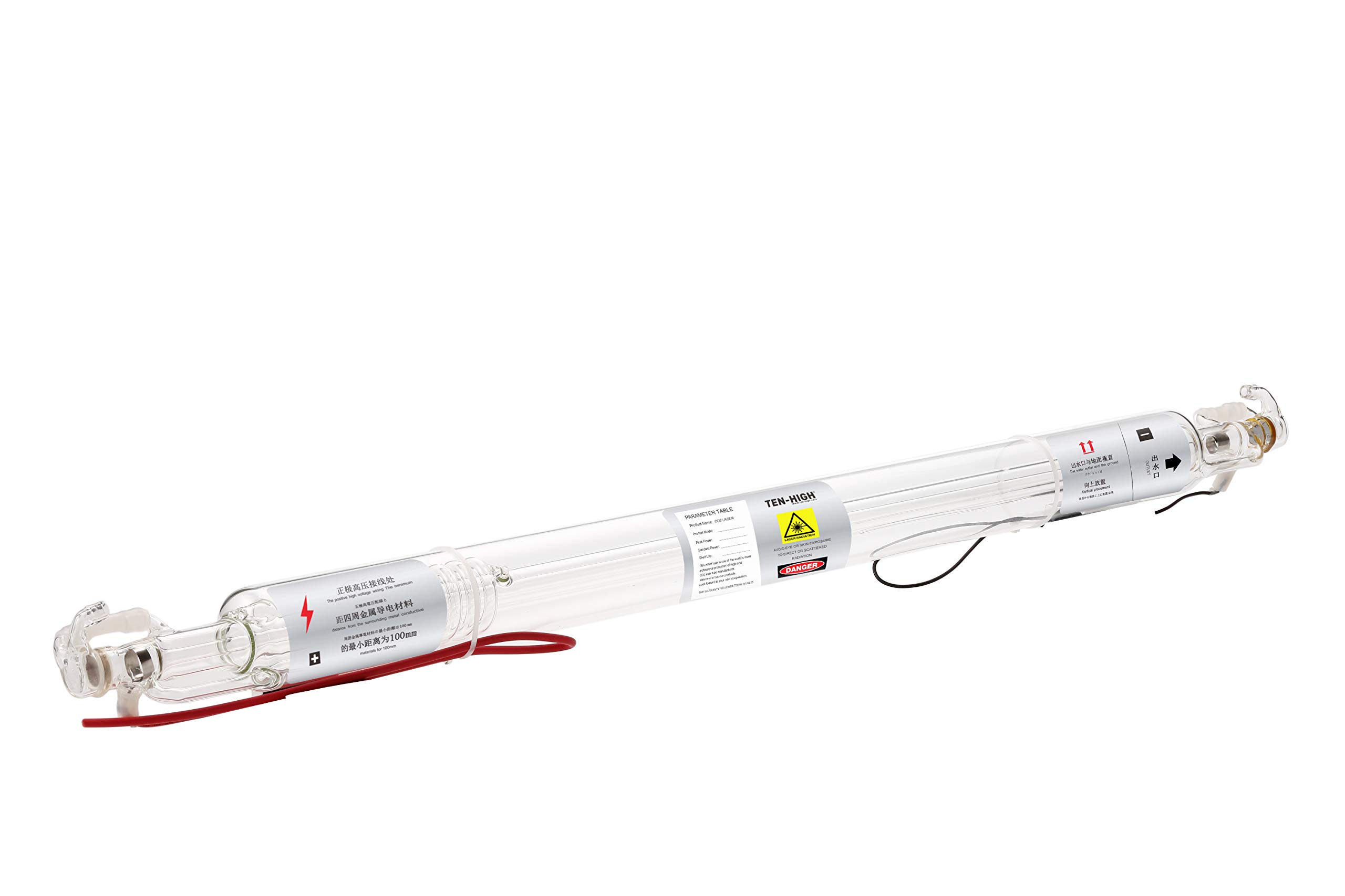
In a conventional CO₂ laser this nitrogen is excited by running an electric discharge through the gas. This is how most commercial CO₂ laser tubes you can find online work, and it is for good reason. This method is excellent at creating cheap, compact, high power lasers. Today on eBay you can buy a 200 watt CO₂ laser which can cut anything from metal to wood for under a few hundred dollars. However, if you truly want to scale beyond a few hundred watts to a few kilowatts you need to move past electric discharge to a method which can create population inversions in denser gases, can reject heat more efficiently, and does not require high power electronics; that is where the gas dynamic laser comes in.

Thermal Population Inversion

Imagine for a second that you have an amazing microscope which can zoom in on individual molecules in a box and observe each of their behavior. If you were to watch the molecules' behavior as you heated up a box of monatomic helium atoms you'd observe roughly the classically expected behavior of a perfect gas. Mainly the molecules would accelerate (on average) as the gas heats up, moving faster and faster in accordance with the temperature of the gas.

Now instead imagine if you had a box of a diatomic molecule, like N₂, and slowly increased the heat. Sure you would observe some of the same behavior as helium, seeing the molecules gradually bounce around faster and faster, but you would also see other effects as well. As the molecules bounce around they'd start rotating faster and faster and even start vibrating. In physics these extra ways a molecule can move around are known as degrees of freedom, and increase with the number of bonds in a molecule.

The reason this matters is captured by the equipartition theorem, which states that in thermal equilibrium every active degree of freedom stores, on average, the same amount of energy: $\tfrac{1}{2} k_B T$ per molecule. For a gas of $f$ degrees of freedom this gives a molar internal energy of

$U = \frac{f}{2} R T$

where $R$ is the universal gas constant. The molar heat capacity at constant volume, $C_V$, is simply how much this internal energy changes per degree of temperature:

$C_V = \left(\frac{\partial U}{\partial T}\right)_V = \frac{f}{2} R$

So heat capacity scales linearly with the number of degrees of freedom. Helium, being a monatomic gas, can only store energy in its three translational directions of motion ($f = 3$), giving

$C_V^{He} = \frac{3}{2} R$

Nitrogen, on the other hand, has those same three translational degrees of freedom plus two rotational ones ($f = 5$) at moderate temperatures, so

$C_V^{\mathrm{N}_2} = \frac{5}{2} R$

The extra rotational degrees of freedom mean it takes more energy to raise the temperature of N₂ by one degree than it does for helium — some of the energy you add gets siphoned off into spinning the molecules rather than speeding them up. At still higher temperatures the vibrational mode of N₂ begins to activate, adding two more degrees of freedom (one kinetic, one potential) and pushing $C_V$ toward $\tfrac{7}{2} R$.

Using this equipartition theorem, along with the various energy levels of the CO₂ molecule from the previous section, we can now rederive the Boltzmann distribution previously mentioned and prove that a thermal population inversion is impossible.

First we need a model for what a vibrational mode actually is. Each of the normal modes we met earlier — the symmetric stretch, the bend, and the asymmetric stretch — behaves like a tiny quantum harmonic oscillator: a set of atoms oscillating on a spring, but with the catch that quantum mechanics only permits it to hold energy in discrete, evenly spaced rungs. If a mode vibrates with frequency $\nu$, then its allowed energies are:

$E_n = n h \nu, \qquad n = 0, 1, 2...$

where $n$ counts how many quanta of vibration the mode is holding (we ignore the constant zero-point energy, since it cancels out of everything that follows).

Now imagine a huge collection of these oscillators sharing a fixed pool of energy quanta, free to swap them back and forth during collisions. We want to know the most likely way for that energy to be distributed: how many molecules end up with zero quanta, how many with one, how many with two, and so on. A quick check of any statistical mechanics textbook would tell you that the population of any one level falls off exponentially with energy:

$N_n \propto e^{-E_n / k_B T}.$

On a macro scale this tells us how much of each vibrational mode is represented in a fixed quantity of a gas; on the microscale, this tells us for any one gas what the "probability" is that we would find it in any one state. While the above is nice, it does not tell us anything unless we can normalize the probabilities. In other words, in order to have a useful metric of proportion we need to find some normalizing constant to divide each $e^{-E_n / k_B T}$ term by to actually get a set of proportions which all add up to one.

Luckily for us this task is made a lot easier by the fact that each energy level is equally spaced in energy. This simple fact turns what would be a very difficult problem into a simple geometric sum^[1]:

$Z = \sum_{n=0}^{\infty} e^{-n h\nu / k_B T} = \frac{1}{1 - e^{-h\nu/k_B T}},$

this tells us that the fraction of molecules sitting in level $n$ is $N_n / N = e^{-n h\nu/k_B T} / Z$. Take the ratio of any level to any other and the partition function cancels, leaving exactly the Boltzmann factor I asserted at the very start:

$\frac{N_{upper}}{N_{lower}} = \exp\left(-\frac{\Delta E}{k_B T}\right).$

We have now derived it from the energy levels rather than pulling it out of thin air. And with it in hand the impossibility of a thermal population inversion becomes plain. The laser transition we care about runs between two different modes: the asymmetric stretch (the upper laser level, at energy $E_{001}$) and the symmetric stretch (the lower level, at $E_{100}$). At a single temperature $T$ their populations are

$\frac{N_{001}}{N_{100}} = \frac{g_{001}}{g_{100}}\,\exp\left(-\frac{E_{001} - E_{100}}{k_B T}\right),$

where the $g$'s account for the degeneracy of each level. Since the upper level genuinely sits higher in energy, $E_{001} > E_{100}$, the exponent is negative and the upper level is always less populated than the lower one, for every finite positive temperature you could possibly choose. To flip the inequality you would need $T < 0$ — the "negative temperature" we encountered earlier. Heating the gas, no matter how violently, can never produce an inversion.

The crucial word in that argument, though, is single. Everything above assumed that one temperature $T$ governs every mode at once, which is precisely what equilibrium means. The entire trick of the gas dynamic laser is to break that assumption: to drive the slow-relaxing asymmetric stretch to a higher effective temperature than the fast-relaxing symmetric stretch, so that the two modes are no longer described by the same $T$ at all.

Generally things that move slowly and change temperature gradually can be assumed to be in perfect equilibrium, however when flows start moving fast enough these assumptions break down. In fact, one of the (many) lines between "supersonic" and "hypersonic" flows is the velocity at which the assumptions of chemical and vibrational equilibrium break down. It is these exact complications which make hypersonics so hard we wish to exploit to create a seemingly impossible population inversion.

The key observations that ultimately led to the development of the Gas Dynamic Laser come from Arthur Kantrowitz's work on vibrational nonequilibrium in the 1940s. Studying rapidly expanding flows, Kantrowitz showed that a gas can fall out of internal equilibrium: the vibrational energy of molecules relaxes far more slowly than their translational and rotational energy, requiring many molecular collisions to adjust to a new temperature. He called this effect "heat-capacity lag," and demonstrated that in a sufficiently fast expansion the vibrational populations effectively freeze, lagging behind the rapidly cooling flow^[2]. It is precisely this freezing of the slow-relaxing CO₂ and N₂ vibrational modes during a supersonic expansion that a gas dynamic laser exploits to lock in a population inversion. In fact, even the seminal Kantrowitz work on this subject was based on observing this non-equilibrium effect in CO₂.

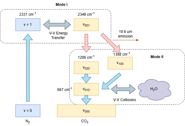
From empirical observations it can be shown that generally in a mixture of CO₂–N₂ gas expanded at high velocity through a converging–diverging nozzle, a "three temperature system" forms, where three different modes act at different temperatures due to differences in vibrational relaxation times as follows:

• An "upper" Mode I, which includes the upper vibrational mode of N₂ and $\nu_{001}$ of CO₂ in equilibrium with each other due to their close energies, but out of equilibrium with the rest of the modes.
• A "lower" Mode II, representing all the lower levels of CO₂ in equilibrium with each other but not with any outside modes.
• The base "translational" temperature, which is the temperature of the classical kinetic movement of the molecules.

What matters dynamically is how long a molecule lingers in each mode before its energy is passed along. We can summarize this with two average lifetimes: $\tau_I$, the lifetime of the upper Mode I (the N₂ reservoir feeding the asymmetric stretch), and $\tau_{II}$, the lifetime of the lower Mode II as it drains down into the translational bath^[2]. The upper mode relaxes far more slowly than the lower, $\tau_I \gg \tau_{II}$, and it is exactly this imbalance — the slow upper reservoir refusing to dump its energy as fast as the lower one empties — that lets the two temperatures separate.

We can now stitch these relaxation times together with the quantum harmonic oscillator math from before to work out exactly how a non-equilibrium gas mixture can be attained. Each of the three modes still carries a mixture of oscillators each with their own distribution, however unlike the previous case now we have three different temperatures we have to contend with instead of just one. The upper laser level (the asymmetric stretch, frequency $\nu_3$, the $001$ level) sits in Mode I at temperature $T_1$, while the lower laser level (the symmetric stretch, $\nu_1$, the $100$ level) sits in Mode II at temperature $T_2$. The rate at which each of these modes decays down to equilibrium with the base "translational temperature" can be described using the Landau–Teller model, that being that the rate at which each of these temperatures decays is roughly:

$\frac{de_n}{dt} \propto \frac{(e_n^{eq} - e_n)}{ \tau_n}$

Where $e_n$ is the average vibrational energy stored in the $n$th mode. Reusing the harmonic-oscillator partition function $Z = (1 - e^{-h\nu_n/k_B T})^{-1}$ from before, this is just the energy-weighted average over the Boltzmann-populated rungs of a single oscillator of frequency $\nu_n$ at its own temperature $T$:

$e_n = \frac{1}{Z}\sum_{k=0}^{\infty} k\, h\nu_n\, e^{-k h\nu_n / k_B T} = \frac{h\nu_n}{e^{h\nu_n / k_B T} - 1}$

(The stat-mech-literate among the audience might recognize this as the Bose–Einstein occupation of a quantum oscillator.)

Now the expression above is the energy of a single oscillator. To understand how this would work in the simulation of a bulk gas, we actually want the vibrational energy held per unit mass of the gas mixture. Converting from "per molecule" to "per kilogram of mixture" introduces two factors for each mode: the number of molecules of that species per kilogram, which turns out to be the species' specific gas constant divided by Boltzmann's constant, and the mass fraction $c_s$ of that species, since only part of the mixture's mass is CO₂ or N₂. The lone $k_B$ that drops out simply rescales each vibrational quantum $h\nu$ into its characteristic temperature $\theta = h\nu/k_B$, which is what naturally pairs with a specific gas constant to give an energy per unit mass.

Summing over every vibrational mode and grouping them by the three-temperature picture:the asymmetric stretch riding along with the N₂ reservoir in Mode I at $T_1$, the symmetric stretch and the doubly-degenerate bend ($g_2 = 2$) sitting in Mode II at $T_2$ — gives the specific vibrational energy of each mode group:

$e_{\mathrm{I}} = c_{\mathrm{CO}_2} R_{\mathrm{CO}_2}\, \frac{h\nu_3 / k_B}{e^{h\nu_3/k_B T_1} - 1} + c_{\mathrm{N}_2} R_{\mathrm{N}_2}\, \frac{h\nu_{\mathrm{N}_2} / k_B}{e^{h\nu_{\mathrm{N}_2}/k_B T_1} - 1}$

$e_{\mathrm{II}} = c_{\mathrm{CO}_2} R_{\mathrm{CO}_2}\left[ \frac{h\nu_1 / k_B}{e^{h\nu_1/k_B T_2} - 1} + \frac{2\, h\nu_2 / k_B}{e^{h\nu_2/k_B T_2} - 1} \right]$

where $c_s$ is the mass fraction of species $s$ and $R_s = R/M_s$ its specific gas constant.

Plugging each of these back into the Landau–Teller relaxation equation above closes the loop: the temperatures $T_1$ and $T_2$ fix the mode energies through the Boltzmann distribution, and the Landau–Teller terms then dictate how fast those energies decay down to equilibrium in a fast moving gas.

The inverse can be computed using methods such as Newton's method. Given these relations of energy to temperature, once we have simulated how much energy is in each level we can then find the temperature and occupancy of each mode, thus telling us exactly when population inversion starts.

Putting this together with basic quasi-1D compressible flow equations, we can then build a basic simulation to determine how to actually attain a population inversion.

Simulation

The analysis above tells us that a population inversion is possible and how we can build a model to simulate it, but to actually design a useful system and find out exactly what gas mixtures and nozzle expansion ratios work, we need a simulation. To that end I wrote a small solver, GDLDesigner, which models the quasi-1D steady-state compressible flow through a converging–diverging nozzle including the two-temperature vibrational non-equilibrium effects that make the whole device work.

The model treats the flow as quasi-1D: every quantity is assumed uniform across a given cross-section and varies only along the nozzle axis $x$, with the local area $A(x)$ entering as a prescribed function. This is generally a canonical method of solving for flow in rocket nozzles which any rocket enthusiast would be familiar with.

Governing Equations

The solver integrates a system of five coupled ODEs in the state vector $\mathbf{y} = [\rho, u, T, e_{v,I}, e_{v,II}]$ — density, axial velocity, translational temperature, and the two vibrational energies. Three of these equations are just the usual conservation laws written for a steady, area-varying flow:

$\frac{d(\rho u A)}{dx} = 0, \qquad \rho u \frac{du}{dx} + \frac{dp}{dx} = 0, \qquad h + \frac{u^2}{2} = h_0$

namely conservation of mass, conservation of momentum, and conservation of total enthalpy $h_0$ (the energy equation for an adiabatic flow). The remaining two equations are what set a gas dynamic laser apart from an ordinary rocket nozzle. These equations are then supplemented with the Landau-Teller vibrational relaxation equations for our gas mixture derived above.

$\rho u A \frac{de_{v,i}}{dx} = \rho A\, \frac{e_{v,i}^*(T) - e_{v,i}}{\tau_i}$

Numerical Method

These equations add a bit of a wrinkle into our solver. While normally nice closed form relations can be derived from the quasi-1D flow equations, adding in vibrational non-equilibrium makes a nice closed form equation impossible, requiring a numerical solver for the differential equations. This is where Anderson and my work diverges. Limited by the computers of his time, Anderson chose a time-marching solver, computationally cheaper but less stable^[3]. I on the other hand (with the help of Claude) used a space stepping initial value problem (IVP) solver, integrating the state of the gas step by step along the nozzle axis, trading a bit of computational cost for the stability needed to easily explore a wide variety of design conditions.

To build the space stepping IVP solver the system above is rearranged into five explicit derivatives describing how the five state variables — density $\rho$, velocity $u$, translational temperature $T$, and the two vibrational energies $e_{v,I}$ and $e_{v,II}$ — all evolve as they travel down the nozzle:

$\frac{du}{dx} = \frac{u}{M^2 - 1}\left[\frac{1}{A}\frac{dA}{dx} - \frac{(\gamma_f - 1)}{a^2}\left(\frac{de_{v,I}}{dx} + \frac{de_{v,II}}{dx}\right)\right]$

$\frac{d\rho}{dx} = -\rho\left(\frac{1}{u}\frac{du}{dx} + \frac{1}{A}\frac{dA}{dx}\right), \qquad \frac{dT}{dx} = -\frac{1}{c_{p,\mathrm{tr}}}\left(u\frac{du}{dx} + \frac{de_{v,I}}{dx} + \frac{de_{v,II}}{dx}\right)$

$\frac{de_{v,i}}{dx} = \frac{e_{v,i}^*(T) - e_{v,i}}{u\, \tau_i}, \qquad i \in \{\mathrm{I}, \mathrm{II}\}$

where $a$ is the local frozen speed of sound, $M = u/a$ the Mach number, $\gamma_f$ the frozen specific-heat ratio, and $c_{p,\mathrm{tr}}$ the translational–rotational specific heat. Carrying temperature $T$ as a state variable rather than total energy is what makes this clean: with $T$ in hand the pressure, internal energy, and speed of sound can all be written explicitly, so every right-hand side is a closed algebraic expression that scipy.integrate.solve_ivp can evaluate directly. The two relaxation times $\tau_I$ and $\tau_{II}$ (from the Millikan–White correlations and mixing rules) are recomputed at every step from the local temperature and composition.

The integration is seeded at the reservoir from stagnation conditions: density and temperature from the isentropic stagnation state, velocity from the mass flow rate and local area, and both vibrational energies initialized in equilibrium with the stagnation temperature, $e_{v,i}(x_0) = e_{v,i}^*(T_0)$. That same stagnation state fixes the total enthalpy $h_0$ which is conserved all the way down the nozzle.

To feed the solver realistic inlet conditions there is also a combustion front-end built on Cantera, which works out the stoichiometry and stagnation conditions of the burnt gas for a combustion-driven design. Two reference scenarios ship with the project as configuration files: a direct-heating case reproducing Anderson's textbook treatment^[1], and a combustion-driven case based on Itaya et al.^[3], which lets the model be validated against published results before being trusted on a novel design.

Performance Modelling

The solver hands us the three temperatures: the translational–rotational bath $T$, the upper Mode I temperature $T_I$, and the lower Mode II temperature $T_{II}$, each at every point along the nozzle. The final step is to turn that thermodynamic state into a measure of the energy we could in principle pull out as laser light. The trick is that each temperature fixes the population of its levels through the Boltzmann distribution, so the upper laser level population follows $T_I$ and the lower laser level population follows $T_{II}$. The size of the population inversion is just the difference between the two, and multiplying that inversion density by the energy of a single 10.6 μm photon gives the extractable energy stored per unit volume of gas. Folding in the mass flow then converts this into a laser power. My implementation of this calculation, along with the full flow solver, lives in the GDLDesigner repo.

It is important to be clear about what this number represents: it is a ceiling, not a prediction of real output. The calculation assumes that the entire inversion can be drained to zero and that every available photon is collected, with no optical losses anywhere. A real laser never reaches this and a litany of real world inefficiencies all eat into this output value. The real extractable power will always be some fraction of this theoretical maximum, but the ceiling is still the right quantity to optimize a design against, since a design that cannot produce a large inversion in the first place has no hope of lasing well no matter how good the optics are.

Results

Taking all this together, we can create a complete simulation of a lasers idealized performance from the following design parameters:

• Gas composition (fraction N₂ / CO₂ / H₂O + diluents) or fuel / oxidizer chemistry (computed using Cantera)
• Gas initial temperature (either from direct heating or computed using Cantera combustion simulation)
• Chamber pressure
• Nozzle geometry (function describing nozzle from stagnation condition to exit)

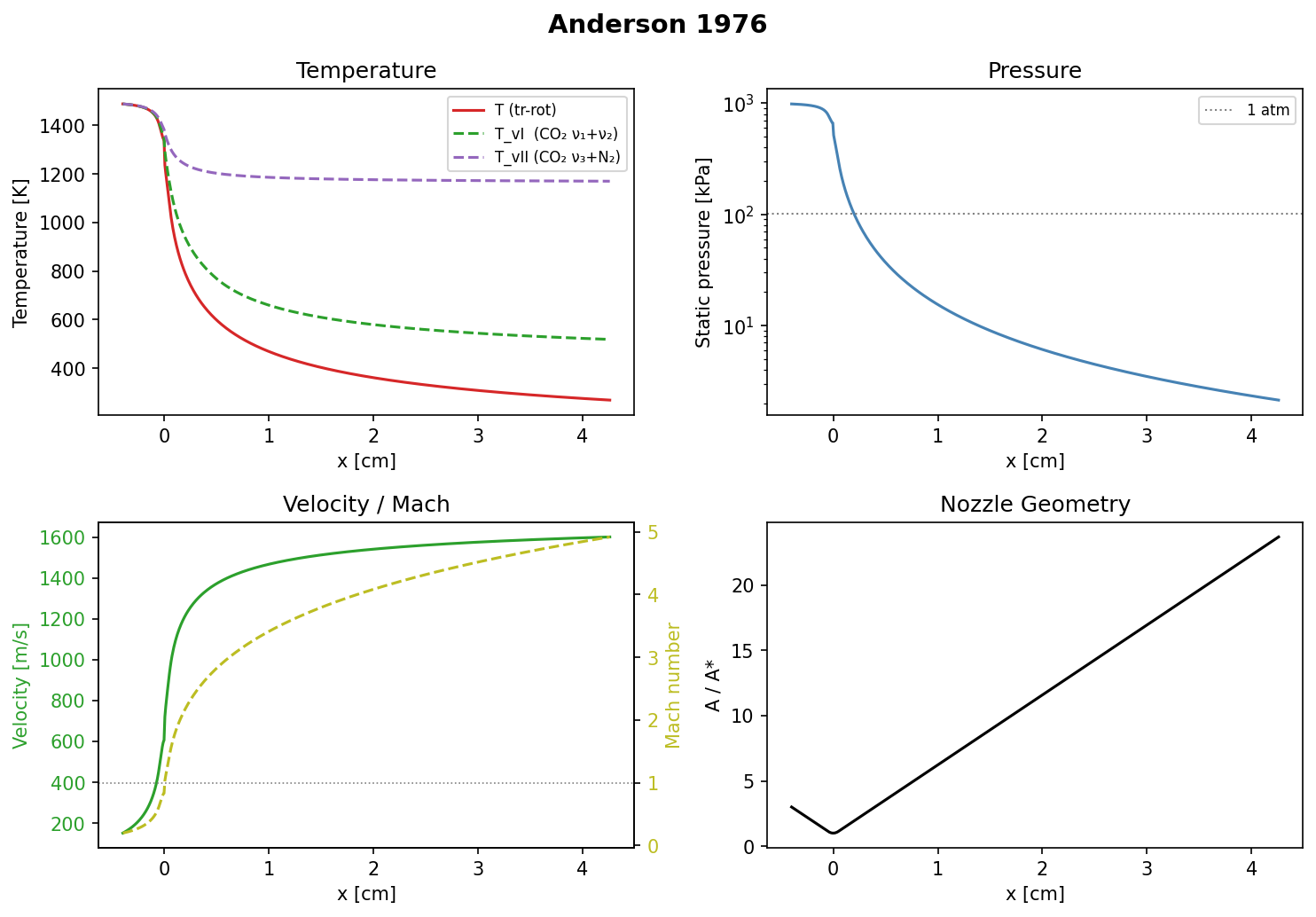
Here is a resulting simulation of a setup of an idealized gas dynamic laser, based on measurements from Andersons work:

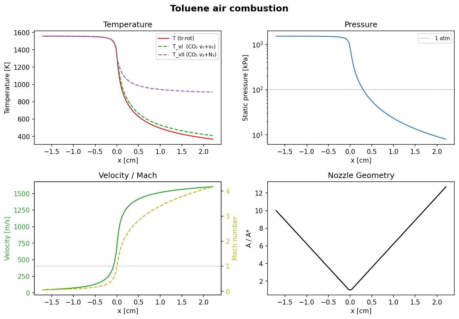
Here is a more modern design based on a system with air toluene combustion:

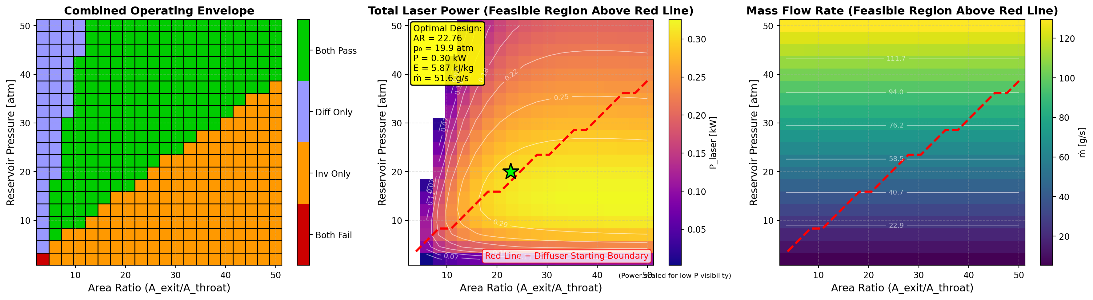
In addition to solving for individual systems, the wealth of compute available today also lets us grid search through design parameters allowing us to find the optimal design for a set of conditions:

A more detailed explanation of the simulation, as well as more configurations, can be found in the GitHub repo.

Limitations

While this work did give a good baseline to work off of, the simulation is still limited. Here are some of the limitations which may be expanded upon in future work:

• Empirically derived rates are still based off of 1960s-era work on the subject. More up-to-date models for vibrational lifetimes may be available.
• The three temperature model does a poor job of accounting for the effect of H₂O and other diluents on the gas such as O₂; a more complex model like a six temperature model may yield more accurate results^[10].
• The model can be expanded to higher dimensions to give a more accurate accounting of performance.
• Current simulations are done on a simple wedge nozzle design; a more optimal nozzle geometry should be used.

Overall the simulation is still limited but provides a solid foundation for my design work.

Design

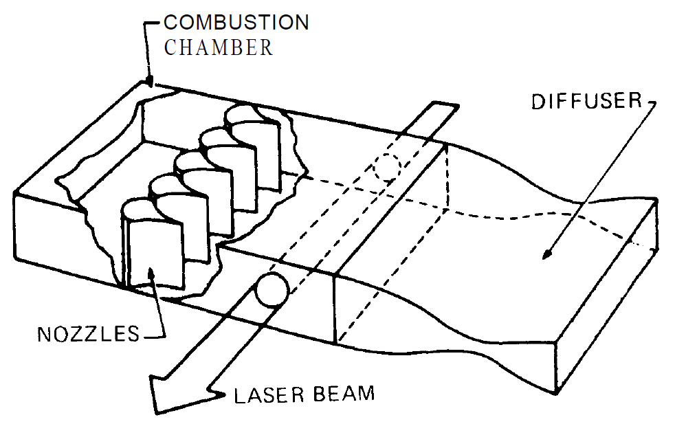
In some sense a gas dynamic laser is just a rocket-powered laser — they share many components such as combustion-powered converging–diverging nozzles and high pressure air–fuel combustion chambers, and thus share many of the same design techniques. However they are not one hundred percent alike; you can't just plug an off-the-shelf motor into some laser optics and go. Whereas a rocket engine wishes to simply maximize the amount of thrust which can be extracted from the fuel mixture, a gas dynamic laser is attempting to coordinate a careful balance of combustion conditions and chemistry coupled into specific flow conditions. As a result, while they can still share a lot of design elements and ideas on the combustor side (I take a lot from the Half Cat Rocketry reference book), anything downstream of the combustor is unique to a gas dynamic laser and has unique design challenges not found in a rocket engine. Still, I took a lot of inspiration from other hobby liquid rocket engine designs as a guide as to what is possible for a hobby designer. While I didn't explicitly take any designs from them, the Half Cat Rocketry design guides were a huge help.

To turn the simulated design into reality four separate components must be designed, each of which have interlinking performance and requirements and numerous sub-components listed here:

• The gas generator
  • Fuel / Oxidizer chemistry
  • Injector design
  • Support fluids system
• Nozzle
  • Nozzle expansion ratio / geometry
  • Throat area
  • Cooling system
• Supersonic diffuser
• Optics
  • Windows
  • Mirrored cavity

As follows I will go through each design component, listing the basic tradeoffs one must make as well as my choice for my homemade design.

Gas Generator

The gas generator system is the most important and interesting aspect of gas dynamic laser design. As shown above, as long as N₂, CO₂ and H₂O can be created at sufficient ratios and temperatures, population inversion can be attained. The amazing thing about this particular mix of gases is that it just happens to be exactly the mixture you get when you burn any hydrocarbon in air! However, there is one catch. The sorts of exhaust mixtures you get from burning a typical hydrocarbon are vastly different than the idealized ratios you want for high performance. Moving away from the ideal ratios of N₂, CO₂ and H₂O can degrade performance and even kill the population inversion altogether. It is this conflict between ease of design and performance which drives some of the more interesting designs proposed historically.

Fuel Choice

The ideal ratio of N₂:CO₂:H₂O by molar ratios is roughly 100:10:1 for maximum laser performance (the precise ideal amount depends on temperature, pressure, and nozzle geometry), while on the other hand burning a typical hydrocarbon in air produces vastly more H₂O and less CO₂ than ideal. For example methane, with a 1:4 carbon to hydrogen ratio burned stoichiometrically with oxygen, results in a CO₂ to H₂O ratio of 1:2, far from the ideal 10:1. Increasing the complexity of the molecule increases the efficiency a little: a saturated long chain hydrocarbon approaches a carbon to hydrogen ratio of 1:2, giving a 1:1 CO₂ to H₂O ratio after being burned. Efficiency can yet still be increased by adding more carbon–carbon bonds to our ideal fuel, with a fuel such as acetylene or benzene having a carbon to hydrogen ratio of 1:1, giving a CO₂ to H₂O ratio of 2:1. Still a far cry from the ideal 10:1 but still a lot better than methane.

Of course, more efficiency can still be found by substituting some of the hydrogens with nitrogen compounds, however then you start running into stability problems. While the ideal fuel from a stoichiometric compound would look something like an aromatic carbon with most of its hydrogens replaced with nitrogen groups, what I just described is TNT, not exactly the most friendly thing to fuel a rocket engine.

The table below collects a handful of candidate fuels, ordered roughly from the easiest and safest to handle toward the most energetic (and most dangerous). Notice how the CO₂:H₂O ratio steadily improves as we trade hydrogen for carbon and then for nitro groups, right up to hexanitrobenzene which produces no water at all:

Fuel	Formula	CO2:H2O (burned in air)	Flame temp. in air	Safety	Toxicity	Notes
Methane	CH4	1:2	~1950 °C	Flammable; explosive in air	Asphyxiant, not toxic	Cheap, ubiquitous; needs pressurized storage
Carbon monoxide	CO	1:0	~2100 °C	Flammable	Highly toxic (binds hemoglobin)	Carries its own oxygen, produces no water; low energy density
Ethanol	C2H5OH	2:3	~1950 °C	Flammable	Low	Cheap, easy to handle; the most benign option
Acetylene	C2H2	2:1	~2500 °C	Flammable; can detonate under pressure	Low (asphyxiant)	Welding gas, widely available; stored dissolved in acetone
Cyanogen	C2N2	1:0	~4525 °C‡	Flammable; one of the hottest flames known	Highly toxic (cyanide)	Produces CO2 + N2 directly with no water; near-ideal but exotic and hazardous
Benzene	C6H6	2:1	~2100 °C	Flammable	Carcinogen	Common solvent; toxicity is the main concern
Toluene	C7H8	7:4	~2050 °C	Flammable	Moderate (CNS depressant)	Widely available; practical aromatic fuel
Trinitrotoluene (TNT)	C7H5N3O6	14:5	~2700 °C†	High explosive; needs detonator	Liver toxin	Regulated; serious handling/legal hazard
Hexanitrobenzene (HNB)	C6N6O12	1:0	~3000 °C†	Sensitive high explosive	Toxic	Lab-only; hard to synthesize, produces no water
Nitrocellulose	~C6H7N3O11	12:7	~2400 °C†	Shock/friction-sensitive; self-ignites when dry	Mild	Guncotton/smokeless powder; degrades over time

Flame temperatures are approximate stoichiometric adiabatic values; in practice reservoir temperatures run lower depending on mixture and heat loss. † For the energetic materials these are approximate self-decomposition / detonation temperatures rather than flame temperatures in air, since they carry their own oxidizer. ‡ Cyanogen's figure is for combustion in pure oxygen; diluted in air it runs much cooler. The nitrocellulose formula varies with degree of nitration.

Beyond the data in the chart there are a few other considerations as well. While generally higher temperature means higher performance, it only goes up to a point. Eventually at too high a temperature CO₂ (around 2300 K) begins to dissociate, resulting in non-equilibrium chemistry downstream which can degrade performance. Additionally, a major constraint on higher performance fuels is handling them. While fuels like HNB and acetylene seem great, their tendency to spontaneously explode limits their usefulness.

For my own personal design I landed on toluene as my fuel of choice. It perfectly straddles the boundary of accessibility, toxicity, and performance by being essentially the highest performing liquid fuel I can buy from the hardware store. This is also a fuel which was commonly used in many historical designs for essentially the same reasons; it's hard to beat toluene in any tradeoff study where safety and fuel accessibility is a concern. Of course this still leaves future room for experimentation, as all of the fuels on the list have been experimentally tried and verified to work in gas dynamic lasers in some form or another. In particular, solid powered gas dynamic lasers using common nitrocellulose (gunpowder) may be another accessible path for hobby creators.

Oxidizer Choice

Compared to the litany of fuel choices oxidizer choice is more mundane. Ultimately the design comes down to tuning the nitrogen to oxygen ratio to maximize performance. This really leads to three practical choices for oxidizers:

• Nitrous oxide: 66% nitrogen, 33% oxygen, higher energy but non-ideal ratio. Self-pressurizing and liquid.
• Air: 80% nitrogen, 20% oxygen, better ratio but lower energy, very low density.
• Custom N₂/O₂ mixture: tuned for fuel choice, best performance but hardest to get.

Ultimately for hobby design the choice is obvious: compressed air is high performance, easy to attain, easy to handle, and most important of all cheap. In a project full of hard problems and tough tradeoffs this is the one welcome reprieve. Even at larger industrial or military scales the obvious upsides of air combustion made it the most obvious option for most historical designs.

Fuel Oxidizer Ratio

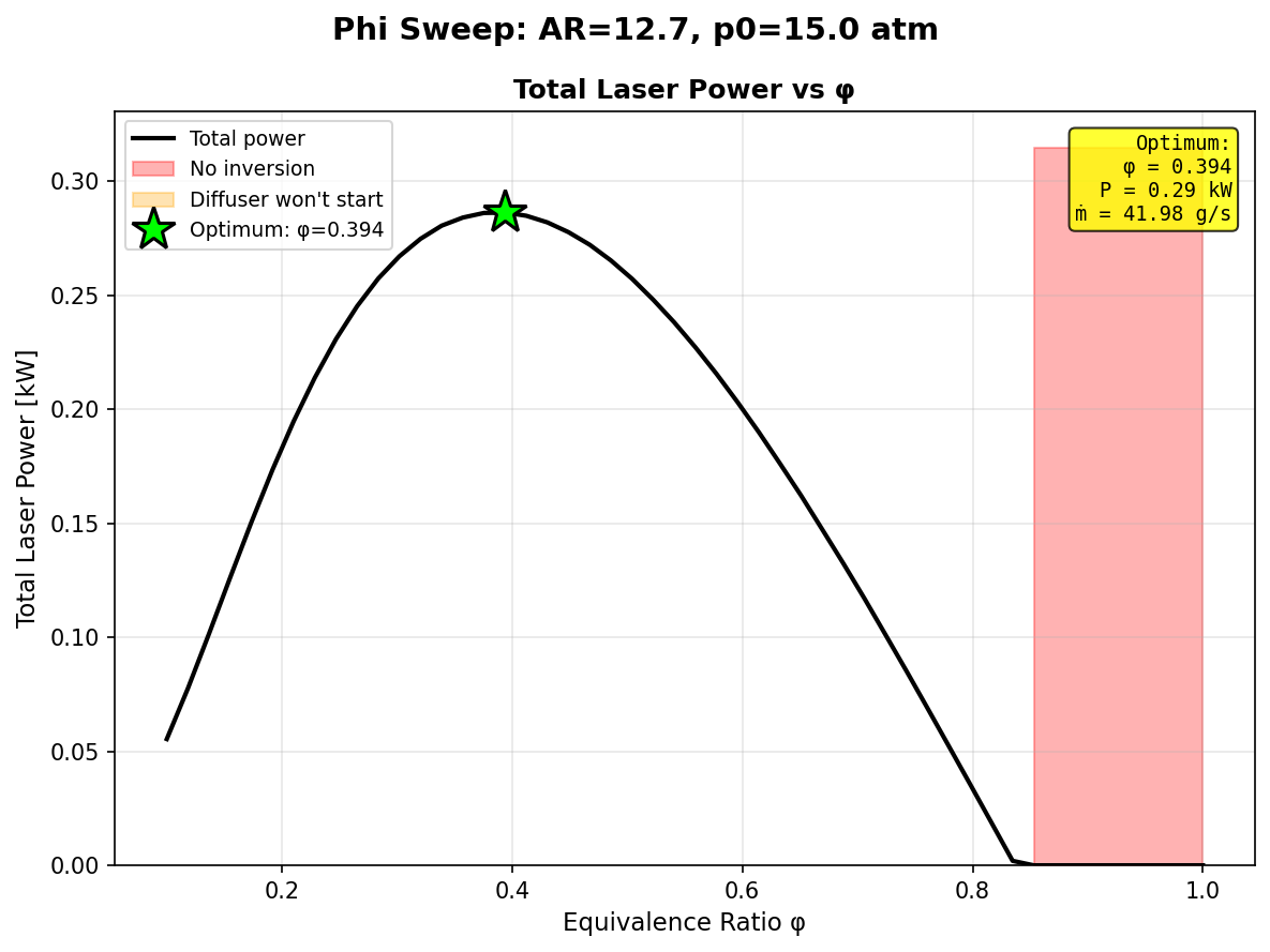
Fuel Oxidizer ratio is another design lever we have to optimize our design which turns out to be quite useful. Varying the fuel air ratio of our combustion from the stoichiometric value ($\phi=1$) yields some important tradeoffs for creating an optimal design mainly:

• Reducing reservoir temperature
• Increasing nitrogen ratio
• Adding in more diluents (extra oxygen for air rich, various carbon compounds for fuel rich)

It is difficult to account for the effects of all of these, especially the presence of diluents which could affect kinetic rates and optics in ways that are difficult to capture in our simplified model, but I found that an ox rich design generally is easier to design for due to the lower reservoir temperatures and more favorable nitrogen to carbon dioxide ratio.

Desiring a lower reservoir temperature may seem contradictory to the previous statements that laser performance scales with temperature, which is true in a general sense. However, higher temperature drive stricter requirements for our nozzle design in order to achieve population inversion. Which in turn drives harder requirements for manufacturing tolerances and makes it more difficult to efficiently couple our exhaust stream back into the atmosphere with our diffuser.

Chamber Pressure

The final design variable which must be considered in the design of a gas generator system is the chamber pressure. In a typical rocket engine where one wishes to maximize thrust and efficiency you would design for as high a chamber pressure your fluid system and chamber materials would allow for you to go, but in our case the choice is a little more complex. There are two main variables which pull our desired chamber pressure in opposite directions:

• Kinetic rates, which prefer lower chamber pressures
• Diffuser starting conditions, which prefer higher starting conditions

Kinetic rates tend to prefer a lower chamber pressure as higher pressures cause the upper lifetimes to be shortened, reducing the population inversion. Even though the point of the nozzle is in part to cool it down and drop the pressure, the pressure must still maintain a continuous gradient from high to low pressure. Thus a higher pressure chamber results in the exhaust stream spending more time at higher pressure, causing the upper modes to be exhausted faster. The general relationship between pressure temperature and kinetic rates is encoded in an empirical formula known as the Millikan-White equation^[5], which states:

$p\,\tau = \exp\!\left[A\left(T^{-1/3} - 0.015\,\mu^{1/4}\right) - 18.42\right], \qquad A = 1.16\times10^{-3}\,\mu^{1/2}\,\theta_v^{4/3}$

Here $\tau$ is the vibrational relaxation time (in seconds), $p$ the pressure (in atmospheres), and $T$ the local translational temperature. The two parameters that characterize the relaxing pair are $\mu$, the reduced mass of the colliding molecules (in atomic mass units), and $\theta_v$, the characteristic vibrational temperature of the relaxing mode (in kelvin)^[4]. The key consequence for our purposes is that, at fixed temperature, the product $p\,\tau$ is constant — so $\tau \propto 1/p$. Doubling the chamber pressure roughly halves the relaxation time, draining the upper modes faster and eroding the population inversion, which is precisely why kinetic rates pull us toward lower chamber pressures.

On the other hand diffuser performance tends to push our requirements towards higher chamber pressures. A more in depth dive into the ins and outs of diffuser design will come in the later section but in essence the more you expand your exhaust, the more energy you irreversibly lose to entropy across the shock boundary from sonic to subsonic. This tradeoff means that the more you expand the exhaust, the harder it is to bring that exhaust back to atmospheric pressures to effectively run the system without a vacuum system. This means that generally there is a lower limit to your chamber pressure dictated by nozzle geometry and diffuser performance, which for non vacuum pump or active ejector systems is ultimately what will dictate your minimum design chamber pressure.

Nozzle

The nozzle is probably the single most important component for dictating our laser performance while at the same time also requiring the most complex modelling. Every other design decision up and downstream of the nozzle couples into laser performance and drives requirements for nozzle design, thus it is important to understand how the two free variables we have for choosing our nozzle geometry, throat height and expansion ratio drive and are driven by variables across the rest of the system.

In a traditional rocket engine, the one a common hobby designed might make, generally two rough approximations are true:

• Rocket performance per propellant mass is independent of size (i.e. you can approximate the performance solely through area ratios)
• The whole rocket can be designed as rotationally symmetric.

Neither of these cases are true in the case of gas dynamic laser design due to our reliance on non-equilibrium effects.

Unlike a traditional 1D model of a rocket nozzle, the addition of finite non-equilibrium vibrational lifetimes to our model necessitates that our nozzle design necessarily take into account the absolute size of the nozzle, not just the relative sizes. This is because while variables like mass flow rate can scale nicely and evenly with respect to flow area, the lifetimes of our states are fixed variables which do not scale per unit mass. This means that while a nozzle with a 10 mm² throat may experience population inversion, a nozzle with a 10 cm² throat may not, even if all other variables (reservoir pressure, temperature, chemistry) are kept equal.

This can intuitively be explained with some back of the envelope math. Let's say we need our gas to be cooled from maximum temperature to its minimum in under 25 μs in order to create a population inversion. If our gas moves through the expansion part of our throat at an average velocity of Mach 3 (~1000 m/s), then it would mean our nozzle can have a maximum length of 2.5 cm. Given that the average expansion ratio of a gas dynamic laser nozzle is at least 10 or more, this would necessitate that our nozzle area to start with is quite small, on the order of square millimeters, not centimeters.

If under these conditions we were to make a traditional rocket engine style rotationally symmetric nozzle, our total mass flow rate would not be able to surpass a few grams per second, with total laser energies limited to the tens of watts. This is a far cry from the kilowatts or even megawatt power ranges gas dynamic lasers operate best in. Because of this generally instead gas dynamic lasers tend to be designed to operate with a "bank" of thin linear nozzles side by side with very thin total throat heights, down to a millimeter or less. This lets the nozzle expand over a relatively short distance in space while decoupling the beam size (the nozzle width) from the expansion ratio (nozzle height times area ratio). Additionally this has the added bonus of making the whole system relatively expandable, as multiple sections of nozzles can be added to lengthen the beam path, increasing total laser power.

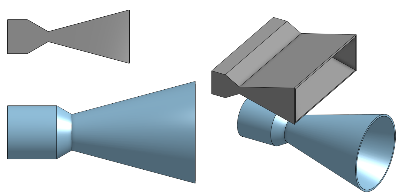
In choosing our design of a linear nozzle, 3 variables must be considered:

• Area ratio
• Nozzle height
• Mass flow rate Each of which must be carefully chosen for a design taking into account all the other subsystems.

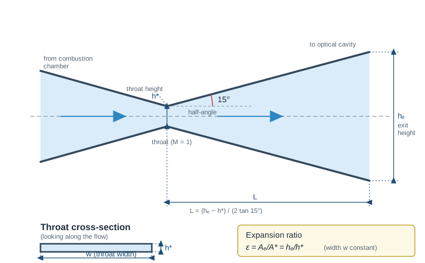
More detail on nozzle design can be found in Anderson's textbook for gas dynamic laser specific designs or any general rocketry reference for more general design advice, this is just meant for a basic overview of the key design aspects for my own gas dynamic laser design.

Area Ratio

For any converging-diverging de Laval nozzle the area ratio, the ratio of the exit area to the throat area, $A_e/A^*$, is one of the most important design variables, as it sets how far the flow expands and therefore how cold and rarefied the gas becomes by the time it reaches the optical cavity. For a steady, isentropic, calorically perfect flow the area ratio is tied directly to the local Mach number $M$ through the area–Mach relation:

$\frac{A}{A^*} = \frac{1}{M}\left[\frac{2}{\gamma+1}\left(1 + \frac{\gamma-1}{2}M^2\right)\right]^{\frac{\gamma+1}{2(\gamma-1)}}$

Once the Mach number is known, the static temperature and pressure follow from the stagnation (chamber) conditions $T_0$ and $p_0$ through the isentropic relations:

$\frac{T}{T_0} = \left(1 + \frac{\gamma-1}{2}M^2\right)^{-1}, \qquad \frac{p}{p_0} = \left(1 + \frac{\gamma-1}{2}M^2\right)^{-\frac{\gamma}{\gamma-1}}$

The key takeaway is that both the static temperature and the static pressure drop as the area ratio grows. As the nozzle area ratio grows, the speed of the exhaust grows as well, which simultaneously cools it and drops its pressure. Note that these closed-form relations assume a fixed ratio of specific heats and an isentropic, equilibrium expansion; in a real gas dynamic laser the vibrational modes freeze out and the flow is not perfectly isentropic, so the actual temperature drop is shallower than these idealized expressions predict (which is why we resort to the full numerical solver above). They nonetheless provide a good intuition as to how nozzle performance is driven by area ratio.

This temperature drop is what primarily motivates the choice of area ratio. Recall that population inversion in a gas dynamic laser is maintained not by pumping the upper level harder, which has its maximum set by the reservoir temperature, but by emptying the lower one. The lower laser level has a thermal floor set by the translational–rotational bath in the ideal case where the bottom is instantly depopulated and the top stays at reservoir temp. Therefore lowering down the temperature of the flow coming out the nozzle is primarily what dictates the performance of our laser. However it is not simply the case that the higher the area ratio the better, once the downstream flow has been sufficiently cooled the lower laser mode will be nearly entirely depopulated, any cooling past that unnecessarily restricts our design.

The way nozzle area ratio drive performance can clearly be seen by sweeping through area ratios for fixed reservoir conditions and simulating the resulting laser energy:

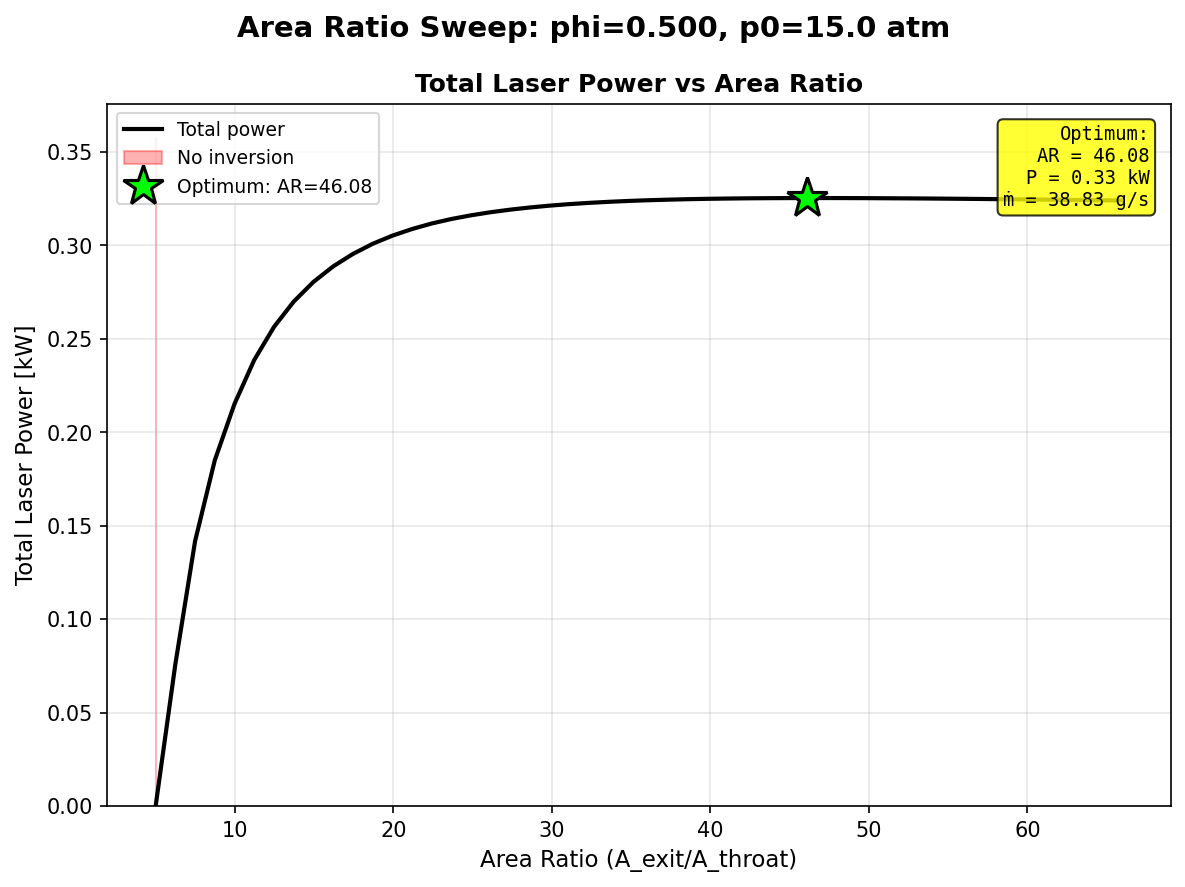
As can be seen the laser performance quickly increases with laser performance to a point, but once the lower level is cooled enough to be depopulated performance then levels off. At very high expansion ratios the performance then starts to decrease as the length of the nozzle increases to the point where the population inversion starts decaying before it even leaves the nozzle. This sweep shows that while nozzle selection is essential to performance, the minimum value needed for a certain level of performance for a given fuel can be determined from some simple simulations where a large set of values can work, and ultimately our design will mainly be constrained by diffuser performance instead.

Nozzle Height

With the area ratio fixed, the throat height becomes the variable that sets the physical length of the nozzle. For a simple wedge nozzle with a 15 degree half angle expansion the geometry is fixed, so the distance needed to reach the chosen area ratio scales directly with the throat height. A taller throat means a proportionally longer nozzle to achieve the same expansion.

As discussed above, the population inversion only lives over a very short distance downstream of the throat before the upper mode relaxes and the gain disappears, a distance that is independent of flow rate. A longer nozzle means the flow spends more time expanding and cooling, which lets the upper mode bleed away before final temperature and pressure is reached. The throat height should therefore be made as small as the manufacturing method will reliably allow, pushing the nozzle as short as possible so that the flow freezes while the inversion is still strong. In practice the lower bound on throat height is set not by the physics but by manufacturing methods and cooling ability.

Mass Flow Rate

The final variable is the total mass flow rate, and conveniently it is almost entirely decoupled from the choices above. Because the throat is choked (the flow reaches Mach 1 there), the mass flow rate is fixed purely by the throat area and the upstream stagnation conditions and not anything downstream of the throat. With the throat height already pinned by the length argument, it is the nozzle width that sets the throat area and therefore the flow rate. Widening the nozzle bank scales the flow rate linearly while leaving the per-slice cooling physics untouched, which is exactly why gas dynamic lasers are built as banks of wide, thin linear nozzles.

For a choked, isentropic, calorically perfect gas the mass flow rate through the throat of area $A^*$ is:

$\dot{m} = A^* \, p_0 \sqrt{\frac{\gamma}{R\,T_0}}\left(\frac{2}{\gamma+1}\right)^{\frac{\gamma+1}{2(\gamma-1)}}$

where $p_0$ and $T_0$ are the chamber stagnation pressure and temperature and $R$ is the specific gas constant of the mixture. The real flow has frozen vibrational modes and is not perfectly isentropic, but the throat sits close to the chamber where the gas is still near equilibrium, so this expression is a good enough approximation for sizing purposes. The significance of this is that the nozzle width is the single knob that sets $\dot{m}$, and once chosen it drives the requirements for every upstream fluid system in combination with the mixture ratios of the propellant and oxidizer.

Geometry Optimization

For my simulation and design I chose to go with the 15 degree half angle wedge nozzle for simplicity's sake, despite it being slightly suboptimal. A more optimal geometry can be generated using techniques such as the method of characteristics (MoC) but that is outside the scope of this post. However one must be careful about what they are optimizing for: typical rocket nozzles optimize for thrust at the cost of nozzle length, whereas in our case we wish to minimize nozzle length at all costs, and don't care much about thrust.

Diffuser

The purpose of the diffuser in our system is a simple one. Immediately coming out of the nozzle the gas is at a pressure significantly below atmospheric and moving at many times the speed of sound; the purpose of a diffuser is to convert a fraction of that kinetic energy back into potential energy to allow the laser system to be smoothly exhausted to the environment.

Out of all the components the diffuser is the most difficult to design but also, in a sense, the easiest to simulate, in part because there is no good way to simulate its performance. To quote J. D. Anderson, "It is important to accept that contemporary supersonic and hypersonic diffuser design is more of an art than a science. This is particularly true for the CO₂–N₂ gasdynamic laser diffuser..."^[1]

As a result most of the following work is more about giving some of the general design heuristics and effective geometries used in the past; to verify any of these, physical testing is required, preferably with a schlieren imaging setup to make really cool images. Much of the practical guidance here, along with the schlieren imagery below, draws on Zerr's experimental study of short diffusers for gas dynamic lasers^[7], which remains one of the more useful hands-on references for the problem.

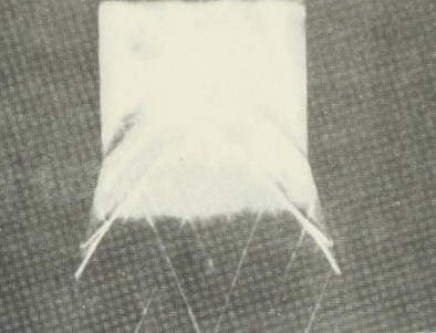
How a Supersonic Diffuser Works

Before getting into any numbers it helps to have a qualitative picture of what is actually happening inside the diffuser. You cannot slow a supersonic flow down to subsonic speeds gently and reversibly; somewhere the flow has to pass through one or more shock waves, and every shock carries an unavoidable loss of total pressure. The crude approach is to let the flow slam through a single strong normal shock, which drops it straight to subsonic but throws away an enormous amount of total pressure. The much better approach, and the one most supersonic diffusers are built around, is the oblique shock train: a converging duct or a series of ramps that turns and compresses the flow through a sequence of weak oblique shocks, each one nudging the Mach number down a little, before a final weak terminal shock takes it subsonic. Because the total-pressure loss across a shock grows steeply with how much the flow is decelerated in a single jump, spreading the deceleration over many gentle oblique shocks recovers far more pressure than one violent normal shock — the same reason it hurts less to walk down a flight of stairs than to jump off the top.

The other concept worth understanding up front is starting. A supersonic diffuser has two possible operating states: an "unstarted" state, where a strong shock sits ahead of or inside the inlet and chokes the flow, spilling and disrupting it, and a "started" state, where the supersonic flow is properly swallowed and the well-behaved oblique shock train sets up inside the duct as intended. A given fixed geometry will only start once the upstream flow is supersonic enough and the back pressure is low enough to push the shock system through and into its design position. This is why diffuser geometry, cavity pressure, and back pressure are all coupled: pick the wrong combination and the diffuser simply refuses to start, the shock disgorges back up into the optical cavity, and the whole carefully-tuned non-equilibrium flow is ruined. A full and very readable treatment of oblique shocks, shock trains, and the starting problem can be found in Anderson's compressible flow text^[6], which is a separate and more general work from the gas dynamic laser book cited throughout the rest of this post.

Pressure Recovery

Despite the empirical nature of diffuser design, we can still bound what is physically achievable. The job of the diffuser is to take the cold, fast cavity flow at static pressure $p_c$ and Mach number $M$ and decelerate it, recovering as much pressure as possible so the exhaust can reach the back pressure $p_b$ (usually atmospheric). The simplest theoretical reference point is a single normal shock followed by an isentropic deceleration to rest. The static pressure jump across a normal shock at Mach $M$ is given by the Rankine–Hugoniot relation:

$\frac{p_2}{p_1} = 1 + \frac{2\gamma}{\gamma+1}\left(M^2 - 1\right)$

but a normal shock is violently lossy in total pressure, and that total-pressure loss is what ultimately limits how much static pressure the diffuser can hand back. The total pressure recovered across a normal shock is:

$\frac{p_{0,2}}{p_{0,1}} = \left[\frac{(\gamma+1)M^2}{(\gamma-1)M^2 + 2}\right]^{\frac{\gamma}{\gamma-1}}\left[\frac{\gamma+1}{2\gamma M^2 - (\gamma-1)}\right]^{\frac{1}{\gamma-1}}$

Real diffusers do not rely on a single normal shock; a well-designed supersonic diffuser sets up a train of weaker oblique shocks that, in principle, throws away less total pressure than one strong normal shock. We capture how well a given diffuser actually performs with a recovery efficiency $\eta_d$, defined as the ratio of its real total-pressure recovery to the ideal normal-shock value at the same inlet Mach number:

$\eta_d = \frac{\left(p_{0,2}/p_{0,1}\right)_\mathrm{actual}}{\left(p_{0,2}/p_{0,1}\right)_\mathrm{normal shock}}$

so that the total pressure delivered to the exhaust is $p_{0,2} = \eta_d \left(p_{0,2}/p_{0,1}\right)_\mathrm{NS}\, p_{0,1}$, and the diffuser successfully exhausts to the environment only when this recovered pressure exceeds the back pressure, $p_{0,2} \ge p_b$.

By this definition $\eta_d > 1.0$ should be attainable — an oblique shock train ought to beat a single normal shock. In practice, however, for the supersonic-to-hypersonic inlet Mach numbers a gas dynamic laser runs at, it is rare to achieve an efficiency above 1.0 at all. Shock–boundary-layer interaction, the thick low-momentum boundary layers that build up along the diffuser walls, flow separation, and the difficulty of keeping a clean oblique shock structure at high Mach number all conspire to drag the real recovery back down toward (or below) the simple normal-shock value. It is therefore safest to design assuming $\eta_d \lesssim 1.0$ and to treat anything better as a pleasant surprise to be confirmed by testing.

For a specific assumed diffuser normal shock efficiency, this relationship determines the absolute minimum reservoir pressure needed to start the diffuser for a specific area ratio. This then dictates the minimum pressure for our combustion chamber, dictating combustion chamber parameters, which in turn dictates nozzle design and thus downstream diffuser performance. This set of relationships is what drives the wheel for our iterative design process.

Design Heuristics

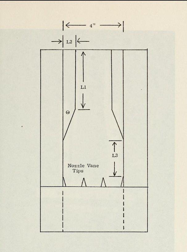
While the specifics of diffuser design come down to trial and error, I take the general design geometry from previous work from Zerr^[7], which generally matches the designs I see throughout the GDL literature. Overall the design of the diffuser is fairly simple, just a flat angled ramp section and a constant area throat. Zerr and Anderson generally suggest an area ratio of throat to nozzle exit of around 0.8; this strikes a balance between having an area large enough to allow the diffuser to start, and acceptable performance. For the ramp angle it appears that a value around 15 degrees is desired. Throat length is the most empirical, and I just chose a value that seemed long enough based on other examples and was simple to manufacture.

Optics

Once the flowing gas carries a population inversion through the cavity, extracting useful light from it is, refreshingly, the one part of a gas dynamic laser that behaves like an ordinary laser. The optical resonator is the same one you would find in any textbook CO₂ laser: there is nothing exotic about it beyond the fact that the gain medium happens to be moving through the beam at hypersonic speed. Because of this I will keep this section brief, a proper treatment of resonator design, mode structure, stability diagrams, and output coupling can be found in standard laser optics text such as Siegman's Lasers^[8], which covers all of it far better than I could here.

The basic job of the optics is power extraction. A pair of mirrors is placed on either side of the flow, their optical axis crossing the gas stream perpendicular to its motion, forming a resonant cavity. One mirror is a maximum reflector that bounces essentially all of the light back into the cavity, while the other is a partially transmissive output coupler that lets a fixed fraction of the circulating power leak out as the usable beam. Photons making round trips between the mirrors stimulate emission from the inverted molecules as they pass, building the intracavity field up until the round-trip gain just balances the losses, at which point the laser is extracting energy from the flow as fast as the gas can deliver it.

Windows

The one genuinely non-trivial optical component is the window that lets the beam out of the pressurized flow duct while holding back the gas. The material has to be highly transmissive at the CO₂ laser's 10.6 μm wavelength, which immediately rules out ordinary glass and narrows the field to infrared materials such as zinc selenide (ZnSe), gallium arsenide (GaAs), or even ordinary sodium chloride (NaCl). On top of the optical requirement the window must survive as a structural part: it has to withstand the pressure differential across the duct, tolerate the thermal load of any absorbed beam power without fracturing or thermally lensing, and resist erosion from the high-speed flow. For more on the mechanical side of mounting and designing optical windows to survive these pressure and thermal loads, see Willistein's tutorial on optical window design^[9]. In general ZnSe windows are widely available due to the common industrial use of CO₂ lasers and are what I would recommend for any home design; however, if you really want to scale power beyond the kilowatt range then no solid window material will work.

For exactly this reason the most powerful gas dynamic lasers historically did away with the solid window altogether, replacing it with an aerodynamic window: a carefully shaped supersonic flow that sustains the pressure difference between the cavity and the outside world while letting the beam pass through nothing but gas, removing any solid material from the high-intensity beam path. This is an elegant but considerably more complex solution, with its own gas-dynamic design problem attached, and a full treatment of it can be found in Anderson^[1]. It is outside the scope of this post, which assumes a conventional solid window.

My Design

Now armed with all this knowledge it is time to build our own laser system. While the information and simulation tools I built can work across a range of exotic systems, our design will mostly be constrained by the ability of a hobby maker to create it for a maximum of a couple thousand dollars. This adds a few limitations which guide the rest of our downstream design:

• No exotic reagents: all fuels and oxidizers safe and accessible
• Medium to low pressure: high pressure fluids systems are dangerous or expensive, generally limiting pressure is safe
• Low mass flow rate: as mass flow rate goes up every fluid system becomes harder and more expensive, with fewer off-the-shelf parts
• All parts small enough to be reasonably cheaply manufactured: don't have the money to machine down hundreds of pounds of feed stock

These general design heuristics get translated into hard requirements for a hobby design:

• Air system must have mass flow rate and pressure low enough to be powered by common welding regulator
• Diffuser dimensions must be compatible with available sheet metal widths
• Laser must couple into atmosphere purely through diffuser with no vacuum system
• Laser optics must use common CO₂ laser cutter optical parts
• Combustion chamber geometry must be compatible with metal 3D printing
• Laser must have at least 100 watts of extractable laser energy

Running these requirements through some test designs and doing a grid search optimization of design parameters landed me on the following basic design:

Parameter	Value	Motivating Requirement
Chamber pressure	15 atm	Print wall thickness and available regulators
Fuel	Toluene	Accessibility and performance
Oxidizer	Air	Accessibility and performance
Air–fuel equivalence ratio	0.5	Derived from simulation
Nozzle expansion ratio	12.7	Common sheet metal thicknesses
Throat height	1 mm	Manufacturing tolerances
Throat width	25 mm	Power requirements and mass flow rate limitations
Combustion chamber manufacturing	Metal 3D printing	—
Diffuser manufacturing	Sandwiched cut sheet metal	—

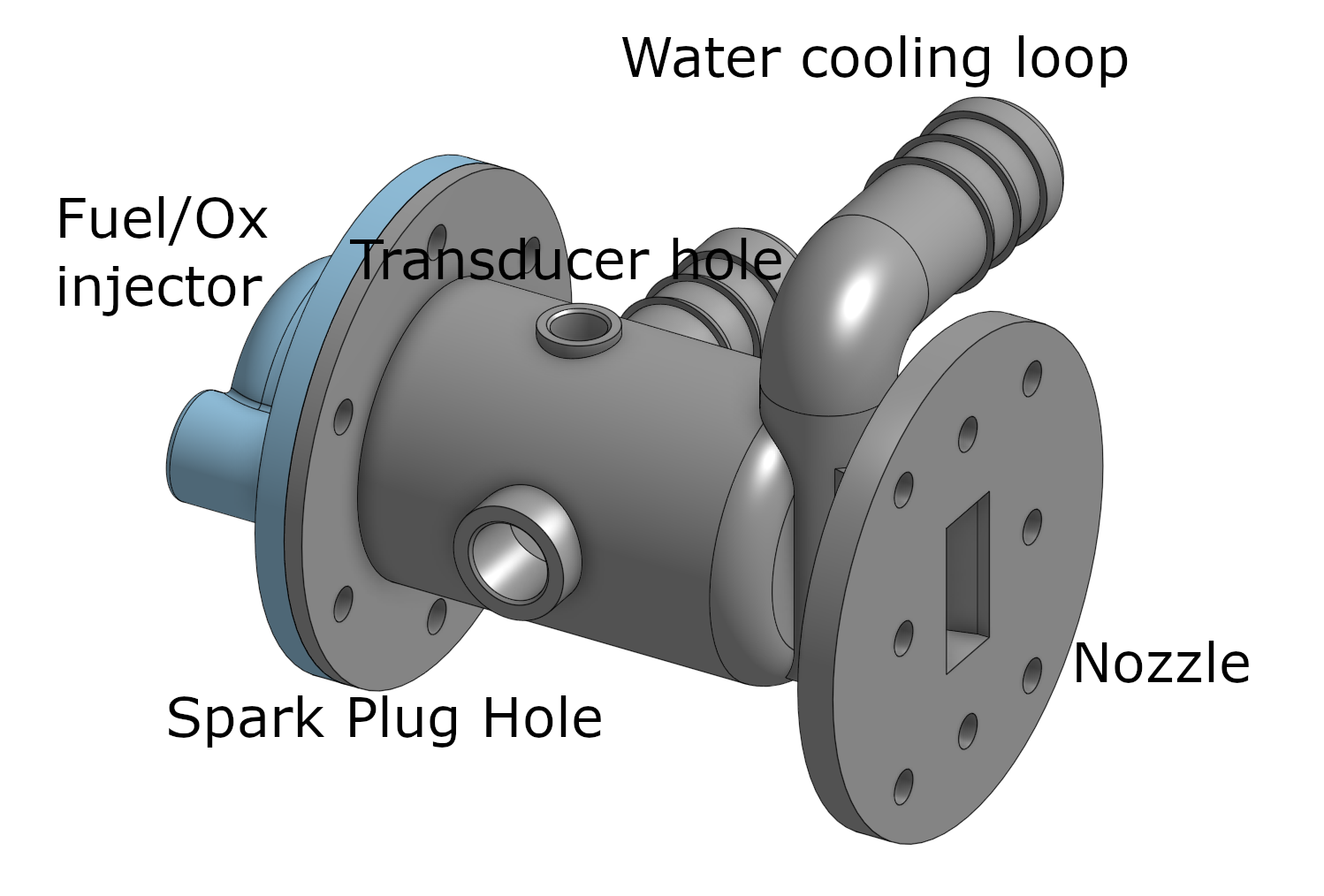
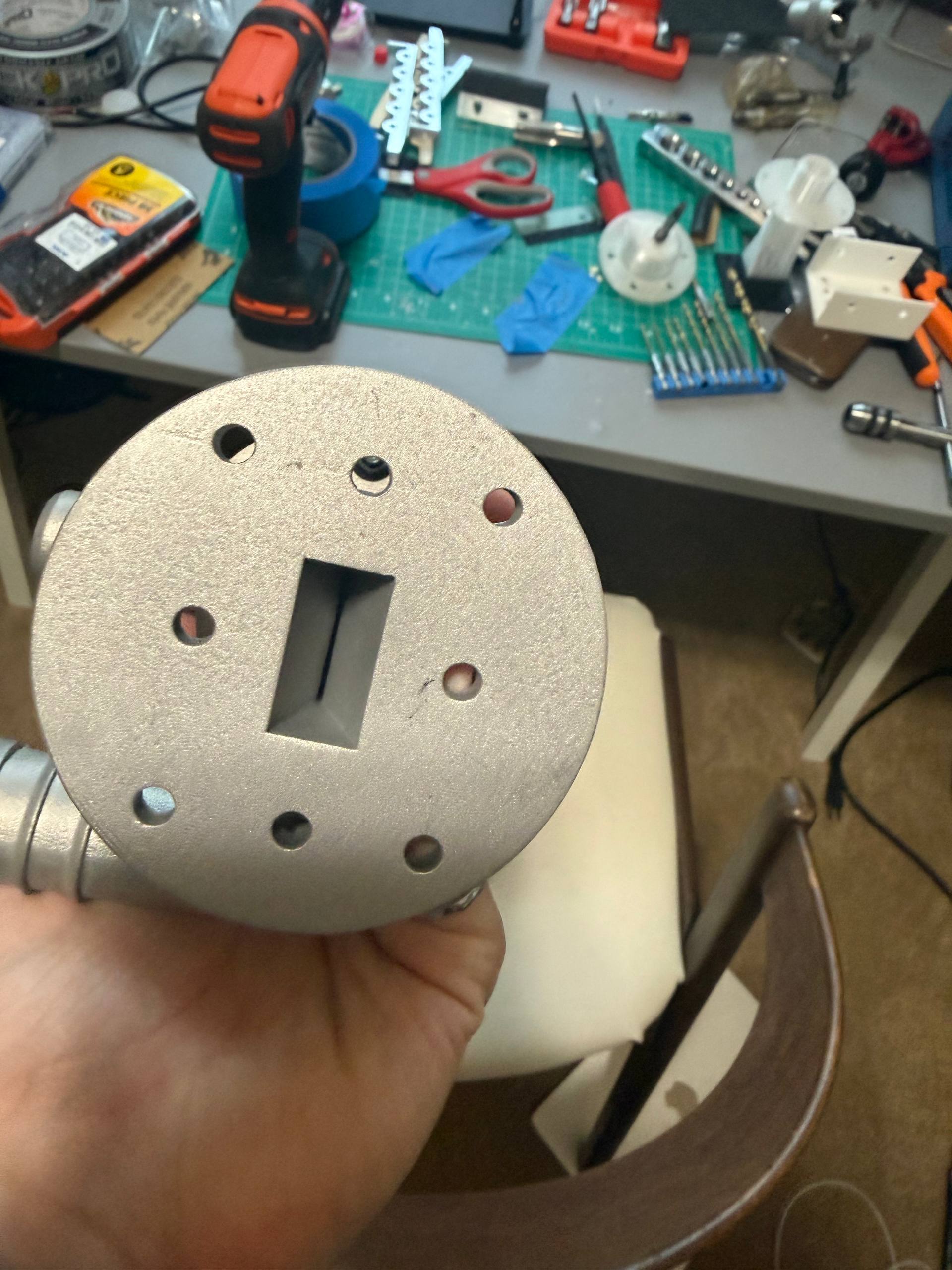
The design and engineering is still a work in progress, but I will add a series of pictures depicting my current progress below.

Design Gallery

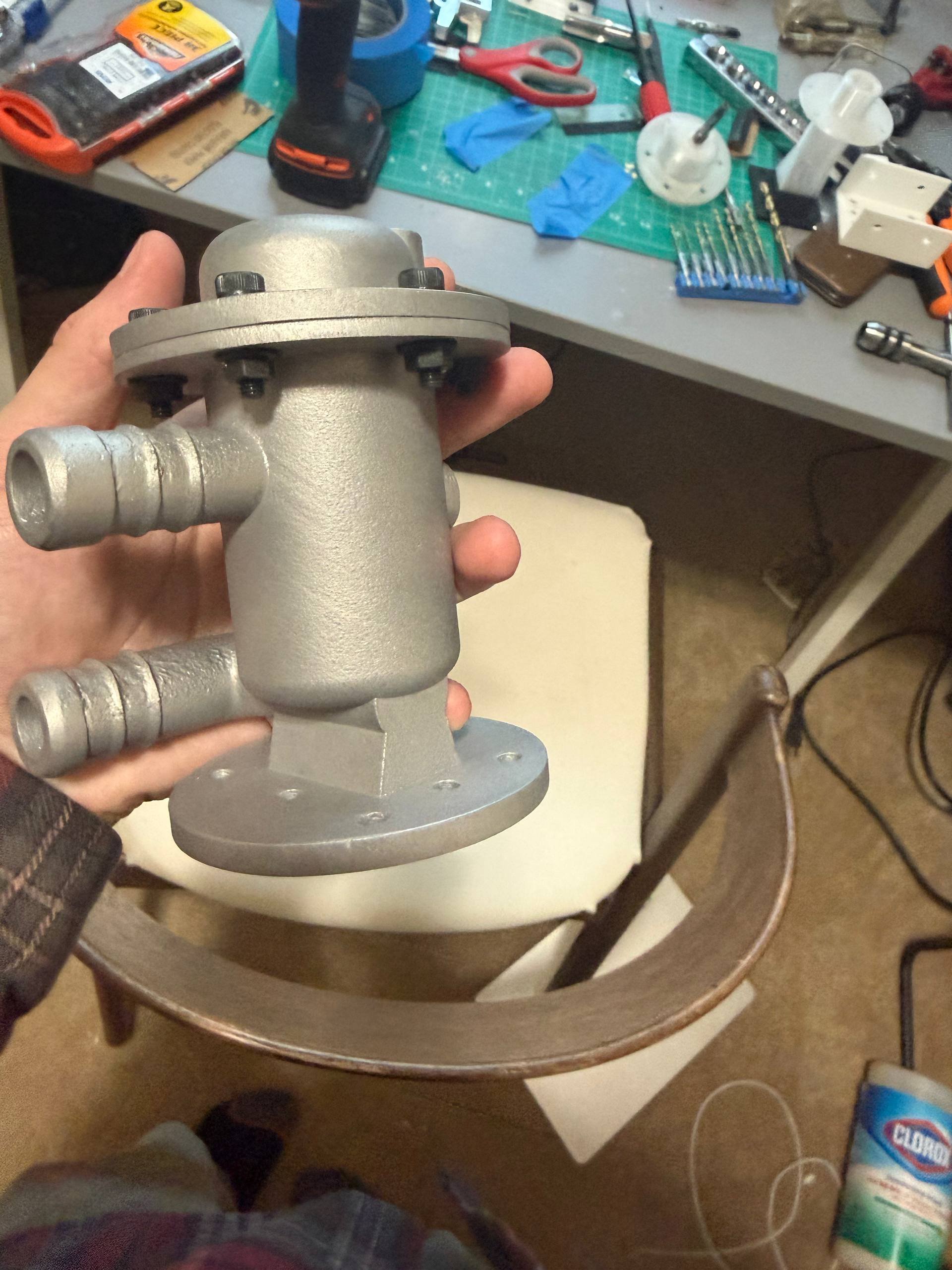
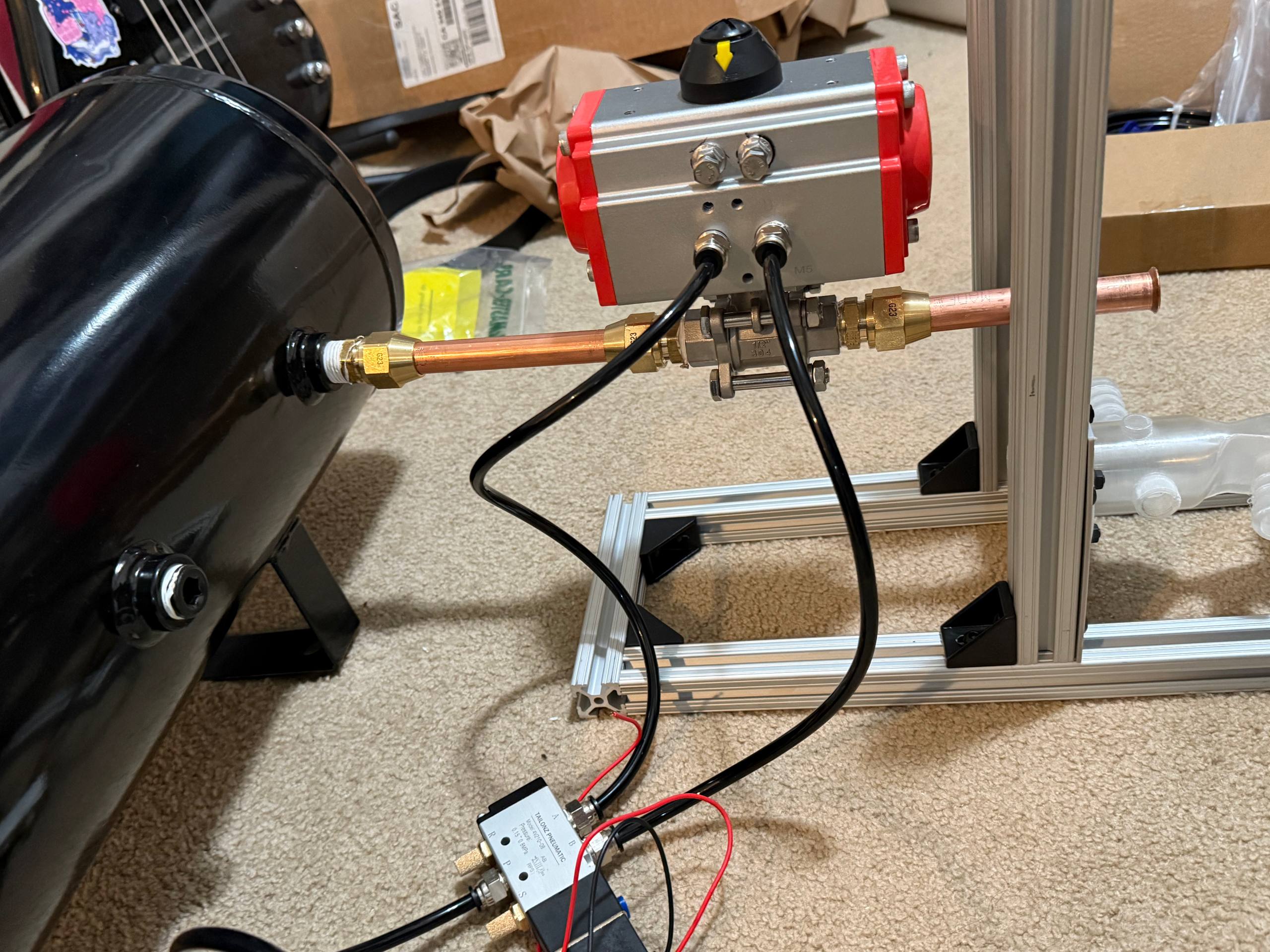
Additional Resources

A collection of resources I found useful that fall outside the scope of this post but are well worth a look if you want to go deeper on any particular subsystem:

• Half Cat Rocketry — an excellent practical resource on liquid rocket design aimed squarely at hobby makers, directly applicable to the combustion and feed systems here.
• Parker O-Ring Handbook (ORD-5700) — essentially required reading for any pressure vessel or sealed-joint design.
• Combustion chamber design equations — a handy reference for the equations governing combustion chamber sizing and performance.
• Small- and medium-output-power CO₂ GDL (SPIE) — an example of other gas dynamic laser systems for comparison.
• Explosion-powered gas dynamic laser (AIAA) — a look at GDLs driven by explosive rather than steady combustion.
• Smokeless powder gas dynamic laser (Quantum Electronics) — a solid-propellant approach to driving a gas dynamic laser.

References

1. J. D. Anderson Jr., Gasdynamic Lasers: An Introduction. New York: Academic Press, 1976.
2. A. Kantrowitz, "Heat-Capacity Lag in Gas Dynamics," The Journal of Chemical Physics, vol. 14, no. 3, pp. 150–164, 1946. https://doi.org/10.1063/1.1724115
3. Itaya et al., "Combustion-driven gas dynamic laser," Proc. SPIE, vol. 3092, 1997.
4. J. D. Anderson Jr., "A Time-Dependent Analysis for Vibrational and Chemical Nonequilibrium Nozzle Flows," AIAA Journal, vol. 8, no. 3, pp. 545–550, 1970. https://doi.org/10.2514/3.5703
5. R. C. Millikan and D. R. White, "Systematics of Vibrational Relaxation," The Journal of Chemical Physics, vol. 39, no. 12, pp. 3209–3213, 1963. https://doi.org/10.1063/1.1734182
6. J. D. Anderson Jr., Modern Compressible Flow: With Historical Perspective, 3rd ed. New York: McGraw-Hill, 2003.
7. J. J. Zerr, "An Experimental Investigation of Short Diffusers for Gas Dynamic Lasers," M.S. thesis, Naval Postgraduate School, Monterey, CA, 1974. https://archive.org/details/experimentalinve00zerr
8. A. E. Siegman, Lasers. Mill Valley, CA: University Science Books, 1986.
9. D. A. Willistein, "An Introduction to Optical Window Design," OPTI 521 Tutorial, College of Optical Sciences, University of Arizona, 2006. https://wp.optics.arizona.edu/optomech/wp-content/uploads/sites/53/2016/10/WillisteinTutorial1.pdf
10. S. A. Losev, "Multi-Temperature Models of Vibrational Relaxation in Gas Dynamic Lasers," in Physical-Chemical Kinetics in Gas Dynamics. Berlin, Heidelberg: Springer, 2013. https://link.springer.com/chapter/10.1007/978-3-642-53962-6_8

Notes

1. This clean geometric sum holds for a single harmonic oscillator with one vibrational frequency. CO₂ is the more complicated case: it has three independent normal modes, each with its own frequency (and the bending mode is doubly degenerate), so the full molecular partition function is a product of three such sums rather than a single one. The argument here is unchanged — every mode still follows its own Boltzmann factor — but the bookkeeping is more involved. See Anderson^[1] for a complete treatment. ↩︎

2. Each of these two effective lifetimes is itself an average over a whole network of individual vibrational relaxation processes, each with its own rate, weighted by the composition of the gas mixture. A more detailed derivation of $\tau_I$ and $\tau_{II}$ from the gas composition and the individual vibrational lifetimes can be found in Anderson^[1]. ↩︎

3. A more detailed treatment of Anderson's original time-marching formulation can be found in his 1970 paper^[4]. ↩︎

4. The Millikan-White correlation is a least-squares fit to a large body of shock-tube relaxation data, and it captures the dominant physics rather than every detail: heavier colliding partners (larger $\mu$) and stiffer, higher-frequency modes (larger $\theta_v$) both relax more slowly, while higher translational temperatures relax faster via the $T^{-1/3}$ Landau-Teller dependence. The correlation is fit per collision pair, so the effective lifetimes $\tau_I$ and $\tau_{II}$ used in the solver are composition-weighted averages over the individual pairwise rates. The fit is least accurate at very low temperatures and for strongly polar or chemically reactive partners, where additional attractive-force corrections are usually applied. See Millikan and White^[5] for the original derivation and tabulated constants, and Anderson^[1] for the more precise rate data and correction factors gathered specifically for validating gas dynamic laser performance. ↩︎